Using Generalised Additive Mixed Models (GAMMs) to predict visitors at Edinburgh & Craigmillar Castles

If you attended my talk on “Generalised Additive Models applied to tourism data” at the Newcastle Upon Tyne Data Science Meetup in May 2019, please find my (more detailed) slides linked below.
Some context
I’d been curious about generalised additive (mixed) models for some time, and the opportunity to learn more about them finally presented itself when a new project came my way, as part of my work at The Data Lab. The aim of this project was to understand the pattern of visitors recorded at two historic sites in Edinburgh: Edinburgh and Craigmillar Castles - both of which are managed by Historic Environment Scotland (HES).
By understand the pattern of visitors, I really mean predict it on the basis of several ‘reasonable’ predictor variables (which I will detail a bit later). However, it is perhaps worth starting off with a simpler model, that predicts (or rather in this case, forecasts) visitor numbers from… visitor numbers in the past. In a sense, this is similar to a classic time series scenario, where we would use the data to predict itself, without resorting to “external” predictors.

Outline
We will begin our discussion by first having a quick look at the data available. Then we will very briefly pause on some modelling aspects, to then have a more meaningful discussion of our data forecast (created in R using package mgcv). Afterwards, we can then discuss the additional sources of data that were used as predictors in a more complex, subsequent model.

The data
Our monthly time series presents itself in long format, and is split by visitors’ country of origin as well as the type of ticket they purchased to gain entry to either of the two sites. Thus each row in the dataset details how many visitors were recorded:
- for a given month (starting with March 2012 for Edinburgh, and March 2013 for Craigmillar Castle, until March 2018),
- from a given country (UK, for internal tourism, but also USA or Italy etc.)
- purchasing a given ticket type (Walk up, or Explorer Pass etc.)
- visiting a given site (Edinburgh or Craigmillar).
To build our first, simpler gamm model, we will collapse visitor numbers across country and ticket type, and only look at variations in the total number of visitors per month for each site. This collapsed data looks like this if plotted in R using ggplot2:
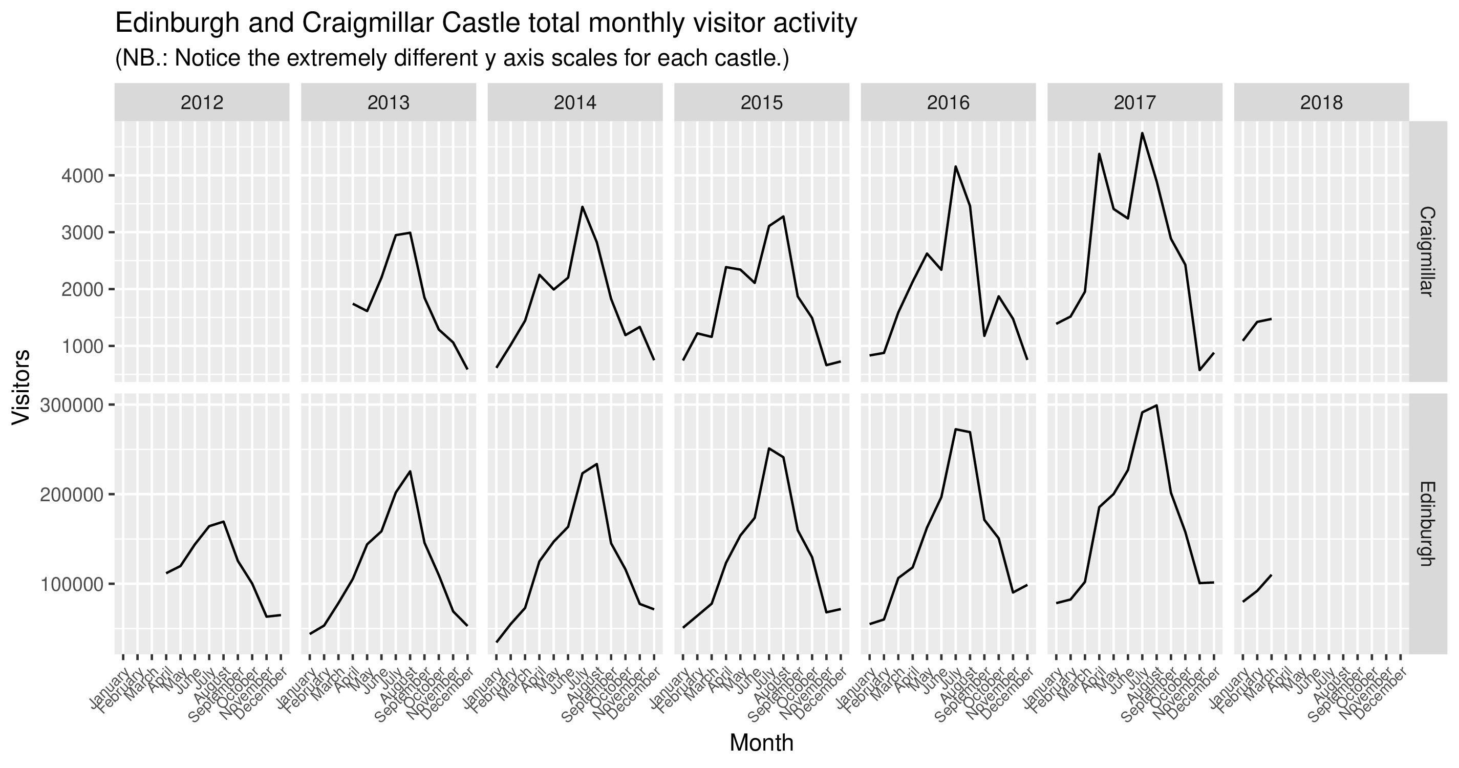
gamm model pick up on these aspects correctly?So what are gamm models? To get a better idea, let’s have a look at where they fit within a conceptual progression relative to other types of models.
Types of models
Regular old linear regression
If trying to predict an outcome y via multiple linear regression on the basis of two predictor variables x1 and x2, our model would have this general form:
- y = b0 + b1x1 + b2x2 + e
Translated into R syntax, a model of this nature could look like:
lm_mod <- lm( Visitors ~ Temperature + Rainfall, data = dat )As the name suggests, this type of model assumes linear relationships between variables (which, as we’ve seen from the plot above, is not the case here!), as well as independent observations - which, again, is highly unlikely in our case (as visitor numbers from one month will have some relationship to the following month).
Generalised additive models (GAMs)
Under these circumstances, enter gam models, which have this general form:
- y = b0 + f1(x1) + f2(x2) + e
As you will have noticed, in this case the single b coefficients have been replaced with entire (smooth) functions or splines. These in turn consist of smaller basis functions. Multiple types of basis functions exist (and are suitable for various data problems), and can be chosen through the mgcv package in R. These smooth functions allow to follow the shape of the data much more closely as they not constrained by the assumption of linearity (unlike the previous type of model).
Using R syntax, a gam could appear as:
library( mgcv )
gam_mod <- gam( Visitors ~ s( Month ) +
                  s( as.numeric( Date ) ) +
                  te( Month, as.numeric( Date ) ) + # But see ?te and ?ti
                  Site,
                data = dat )
However, gam models do still assume that data points are independent - which for time series data is not realistic. For this reason, we now turn to gamm (generalised additive mixed) models - also supported by package mgcv in R.
Generalised additive mixed models (GAMMs)
These allow the same flexibility of gam models (in terms of integrating smooths), as well as correlated data points. This can be achieved by specifying various types of autoregressive correlation structures, via functionality already present in the separate nlme::lme() function, meant for fitting linear mixed models (LMMs).
Unlike (seasonal) ARIMA models, with gamms we needn’t concern ourselves with differencing or detrending the time series - we just need to take these elements correctly into account as part of the model itself. One way to do so is to use both the month (values cycling from 1 to 12), as well as the overall date as predictors, to capture the seasonality and trend aspects of the data, respectively. If we believe that the amount of seasonality may change over time, we can also add an interaction between the month and date. Finally, we can also specify various autoregressive correlation structures into our gamm, as follows:
# mgcv::gamm() = nlme::lme() + mgcv::gam()
gamm_mod <- gamm( Visitors ~
                       s( Month, bs = "cc" ) +
                       s( as.numeric( Date ) ) +
                       te( Month, as.numeric ( Date ) ) +
                       Site,
                     data = dat,
                     correlation = corARMA( p = 1, q = 0 ) )
Forecast model
We can now essentially apply a similar gamm to the one above to our data, the key difference being that we can allow the shape of the smooths to vary by Site (Edinburgh or Craigmillar), by specifying the predictors within the model for instance as: s( Month, bs = "cc", by = Site ), where the bs = "cc" argument refers to the choice of basis type - in this case, cyclic cubic regression splines which are useful to ensure that December and January line up. In our model, we can also add in a main effect for Site.
All this will have been done after standardising the data separately within each site, to avoid results being distorted by the huge scale difference in visitor numbers between sites. At the end of this process, the output we get from our gamm is this:
Family: gaussian
Link function: identity

Formula:
Visitors ~ s(Month, bs = "cc", by = Site) + s(as.numeric(Date),
    by = Site) + te(Month, as.numeric(Date), by = Site) + Site

Parametric coefficients:
              Estimate Std. Error t value Pr(>|t|)
(Intercept)   -0.04312    0.03878  -1.112   0.2687
SiteEdinburgh  0.08738    0.05119   1.707   0.0908 .
---
Signif. codes:  0 ‘***’ 0.001 ‘**’ 0.01 ‘*’ 0.05 ‘.’ 0.1 ‘ ’ 1

Approximate significance of smooth terms:
                                             edf Ref.df      F              p-value
s(Month):SiteCraigmillar                   7.274  8.000 22.707 < 0.0000000000000002 ***
s(Month):SiteEdinburgh                     6.409  8.000 63.818 < 0.0000000000000002 ***
s(as.numeric(Date)):SiteCraigmillar        1.001  1.001 38.212     0.00000000931069 ***
s(as.numeric(Date)):SiteEdinburgh          1.000  1.000 57.220     0.00000000000612 ***
te(Month,as.numeric(Date)):SiteCraigmillar 6.276  6.276  2.935              0.00787 **
te(Month,as.numeric(Date)):SiteEdinburgh   3.212  3.212  3.316              0.02018 *
---
Signif. codes:  0 ‘***’ 0.001 ‘**’ 0.01 ‘*’ 0.05 ‘.’ 0.1 ‘ ’ 1

R-sq.(adj) =  0.913
  Scale est. = 0.081956  n = 132
The output is split between ‘parametric’ (unsmoothed) coefficients, and smooth terms. A key concept here is that of Effective Degrees of Freedom (EDF), which essentially tell you how ‘wiggly’ the fitted line is. For an EDF of 1, the predictor was estimated to have a linear relationship to the outcome. Importantly, mgcv will penalise overly wiggly lines to avoid overfitting, which suggests you can wrap all your continuous predictors within smoothing functions, and the model will determine whether/to what extent the data supports a wiggly shape.
As a measure of overall fit for the gamm model, we also get an Adjusted R-squared at the end of the output (other measures such as GCV - or Generalised Cross Validation - are offered for gam models, but absent for gamm - details in my slides). Judging by this, our model is doing a good job of describing our data, so we can move on to generating a forecast as well… After converting the standardised values back to the original scale, this is how our prediction compares to the raw visitor numbers:
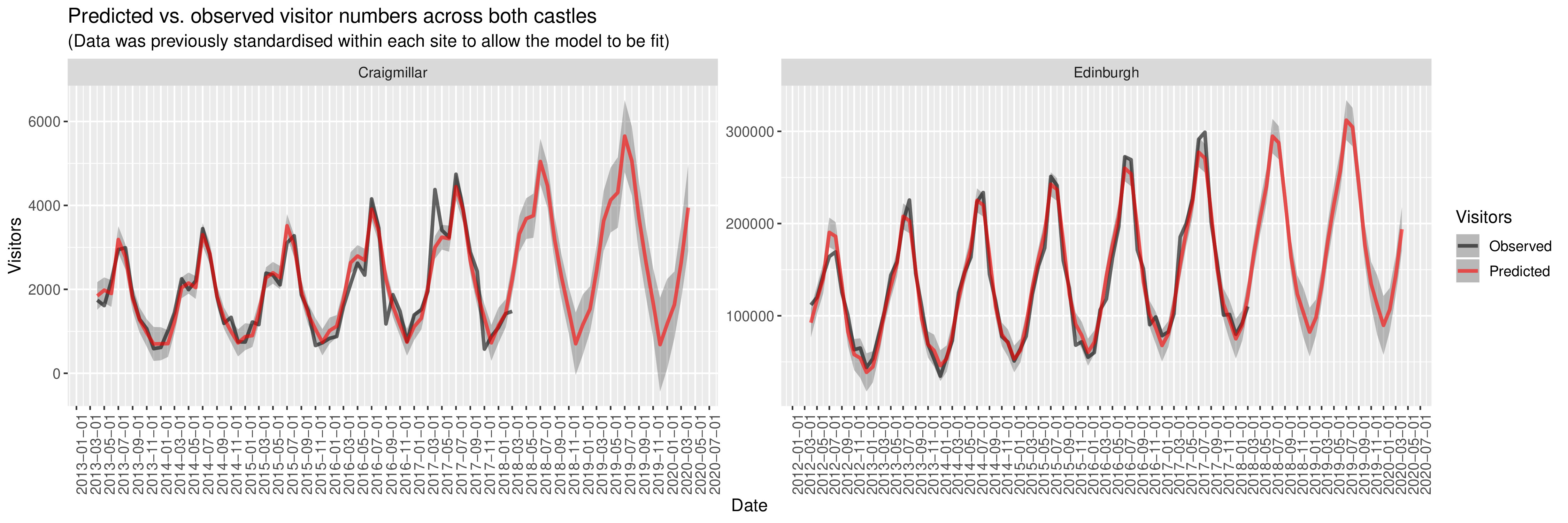
family option in gamm() (perhaps Poisson or Quasi-Poisson), or at least truncating the lower bound of the confidence intervals.Explanatory model
In order to check whether other variables may also contribute / relate to the pattern of visitors we have observed above, several types of data were collected from the following sources:
- The Consumer Confidence Index (CCI) developed by the Organisation for Economic Co-operation and Development (OECD) - this is an indicator of how confident households across various countries are in their financial situation, over time.
- Google Trends R package
gtrendsR- measuring the amount of hits over time and from various countries, for the queries: “Edinburgh Castle” and “Craigmillar Castle”. - Global Data on Events, Language and Tone (GDELT) - this is a massive dataset measuring the tone and impact of world-wide news events as extracted from news articles. Data related to only Scottish events was selected.
- Internet Movie Database + Open Movie Database - these sources were scoured for data on productions related to Scotland (in terms of their plot or filming locations).
- Local weather data
- For-Sight hotel booking data, including information on the number of nights or rooms booked across four major hotels in Edinburgh
These datasets were merged with the HES visitor data by date, (and where applicable) country and site. It was difficult to find datasets covering large intervals of time - hence it was often the case that with every successive data merge, the interval covered would get narrower… So to reduce the chance of overfitting, only one measure per data source was retained for modelling purposes. Variables were selected via exploratory factor analysis (EFA) and by fitting a single factor per data source in order to identify the variable that loaded onto it the highest.
So can these extra predictors explain anything above and beyond the previous, simpler model? Let’s have a look at the final gamm model, which had the following form:
gamm( Visitors ~
      s( Month, bs = "cc", by = Site )  +
      s( as.numeric( Date ), by = TicketType, bs = "gp" ) +
      te( Month, as.numeric( Date ), by = Site ) +
      s( NumberOfAdults ) +
      s( Temperature ) +
      Site +
      TicketType +
      s( LaggedCCI ) +
      s( LaggedNumArticles ) +
      s( LaggedimdbVotes ) +
      s( Laggedhits, by = Site ),

    data = best_lag_solution,
    control = lmeControl( opt = "optim", msMaxIter = 10000 ),
    random = list( GroupingFactor = ~ 1 ), # GroupingFactor = Site x TicketType x Country
    REML = TRUE,
    correlation = corARMA( p = 1, q = 0 )
  )
Based on the output for this model (shown below), we can check in the parametric coefficients section how the various ticket types compare in popularity to Walk Up tickets (used as the baseline category), or how Edinburgh Castle compared to Craigmillar (the latter functioning as the baseline in this case). In the smooth terms section, notably, we have allowed the spline for Date to vary depending on the ticket type concerned - which was useful given the surprising EDF for Membership tickets…
Family: gaussian
Link function: identity

Formula:
Visitors ~ s(Month, bs = "cc", by = Site) + s(as.numeric(Date),
    by = TicketType, bs = "gp") + te(Month, as.numeric(Date),
    by = Site) + s(NumberOfAdults) + s(Temperature) + Site +
    TicketType + s(LaggedCCI) + s(LaggedNumArticles) + s(LaggedimdbVotes) +
    s(Laggedhits, by = Site)

Parametric coefficients:
                        Estimate Std. Error t value Pr(>|t|)
(Intercept)              0.06296    0.06656   0.946 0.344439
SiteEdinburgh            0.22692    0.06350   3.573 0.000372 ***
TicketTypeEducation      0.07420    0.14545   0.510 0.610085
TicketTypeExplorer Pass -0.22165    0.06590  -3.363 0.000804 ***
TicketTypeMembership    -0.43625    0.06684  -6.527 1.14e-10 ***
TicketTypePre-Paid      -0.93159    0.14608  -6.377 2.91e-10 ***
TicketTypeTrade         -0.09395    0.06916  -1.358 0.174698
TicketTypeWeb           -0.10447    0.06915  -1.511 0.131229
---
Signif. codes:  0 ‘***’ 0.001 ‘**’ 0.01 ‘*’ 0.05 ‘.’ 0.1 ‘ ’ 1

Approximate significance of smooth terms:
                                                 edf Ref.df      F  p-value
s(Month):SiteCraigmillar                    4.954928  8.000  7.941 6.94e-15 ***
s(Month):SiteEdinburgh                      7.281621  8.000 20.031  < 2e-16 ***
s(as.numeric(Date)):TicketTypeWalk Up       1.000001  1.000  2.854  0.09149 .
s(as.numeric(Date)):TicketTypeEducation     1.000002  1.000  1.658  0.19821
s(as.numeric(Date)):TicketTypeExplorer Pass 1.000014  1.000  2.690  0.10132
s(as.numeric(Date)):TicketTypeMembership    7.325579  7.326 27.817  < 2e-16 ***
s(as.numeric(Date)):TicketTypePre-Paid      1.000004  1.000  0.231  0.63072
s(as.numeric(Date)):TicketTypeTrade         1.000000  1.000  6.328  0.01206 *
s(as.numeric(Date)):TicketTypeWeb           1.000000  1.000 22.546 2.39e-06 ***
te(Month,as.numeric(Date)):SiteCraigmillar  0.001085 15.000  0.000  0.31354
te(Month,as.numeric(Date)):SiteEdinburgh    5.443975 15.000  2.090 4.26e-07 ***
s(NumberOfAdults)                           1.000009  1.000 40.617 2.93e-10 ***
s(Temperature)                              5.675452  5.675  3.058  0.00436 **
s(LaggedCCI)                                1.000019  1.000  3.921  0.04798 *
s(LaggedNumArticles)                        1.985548  1.986  5.661  0.00598 **
s(LaggedimdbVotes)                          2.702820  2.703  5.187  0.00188 **
s(Laggedhits):SiteCraigmillar               1.000011  1.000  8.012  0.00475 **
s(Laggedhits):SiteEdinburgh                 3.106882  3.107  3.756  0.01092 *
---
Signif. codes:  0 ‘***’ 0.001 ‘**’ 0.01 ‘*’ 0.05 ‘.’ 0.1 ‘ ’ 1

R-sq.(adj) =  0.694   Scale est. = 0.3072    n = 932
You can see this pattern below, in a plot created with the related package itsadug:
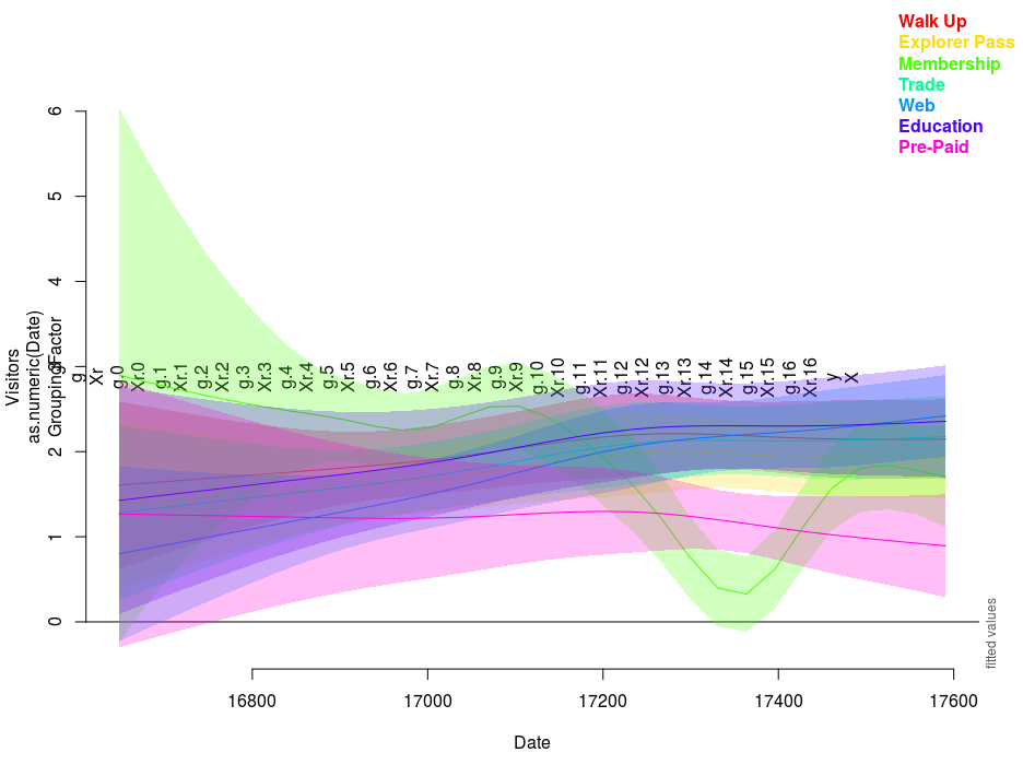
But disappointingly, the Adjusted R-squared for this more complex model is lower than for the previous one - which suggests that the added variables (collectively) are not that successful in predicting visitor numbers at the two castles.
Going further

An important part of building gam or gamm models is carrying out assumption checks - a lot of information about this is present if you consult: ?mgcv::gam.check and ?mgcViz::check.gamViz, with an example also included in my slides here.
Something else that is interesting to consider would be how to validate forecast results. You can check out the idea of evaluating on a rolling forecasting origin or various caveats for time series validation.
Finally, I have only really scratched the surface of gam / gamm models - and so much more is worth exploring. So here are a few great resources you can check out:
- Mitchell Lyons’ introduction to GAMs, which includes an interesting discussion of basis functions and what you can find within
gamobjects in R - Gavin Simpson’s blog
- Noam Ross - Nonlinear Models in R: The Wonderful World of mgcv
- Noam Ross’ Intro Course on GAMs
- Josef Fruehwald - Studying Pronunciation Changes with gamms